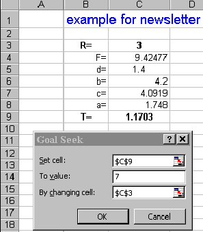
Learn to use “Goal Seek” in EXCEL® SpreadsheetsSuppose you have a messy series of equations (or results) that are linked together. This happens quite a bit in forest sampling. How can you solve for a specific value for one of the parts? Let me give a specific example: (stick with me for a few moments – I am about the make the math go away). R = 3 R is the thing that normally changes by itself, and you are solving for T. If you are really lucky, someone has given you a worked example for the individual equations, so you can check your interpretation of what they mean. Was that “log (Fb)” or “(log F)b ”? R = 3 If you are really, really lucky, they will also give you a spreadsheet so that these equations are perfectly clear. (Always encourage this, and always reward it when it is done). It is a great quality control procedure. Now, suppose that some bozo just has to know what “R” must be to produce a value of 7 for “T”, and assigns you to find out. Maybe he even wants a graph of “R” values for a range of “T”. Time is short, and you have other things to do. The classic response from the math department is to “get all this into one large equation, move the parts around by algebra and solve for R when T=7”. I don’t know how you were at algebra, but I have always found it tedious – although extremely useful. This is not how I want to spend my day. In addition, I am not positive that my solution is correct until I test it by solving all these parts, just to make sure. That usually means setting up these individual equations on an EXCEL® spreadsheet. You could also play around with the “R” value until you came close to 7, because you have spreadsheets to compute the numbers. “Trial and error” methods would get tedious too. Let the computer do the work for you. There is a command in the EXCEL® spreadsheet you should know. Under the “Tools” menu, choose “Goal Seek”. You get 3 boxes to fill in. First choose the cell of the spreadsheet where “T” shows up. In the second box, enter “7”. In the bottom box, fill in the cell where “R” is entered, and choose “OK”. What is inside the cell noted in the bottom box must be a number, not an equation, so the computer can change it. If the computer cannot find a value that changes the result into “7” it will tell you. The computer will now change the “R” value until it finds at least one way to produce T=7 (in some equations, there may be more than one way to produce T=7). In this instance, my computer produced an “R” value of 9.1579 to get a “T” value of 7.000131 – not exact, but close enough for just about any practical purpose. You can change the precision of the spreadsheet by adjusting “Tools/options/calculations” and adjusting “maximum change” or “maximum iterations” (the number of times the computer tries different numbers).
What value of “d” would produce a “c” value of 16? My computer indicates that 5.4742 would do it. All this is entirely without algebra, and can be done with really complex and interrelating equations that will drive you crazy otherwise. Maybe it’s a good idea for somebody to take a look at the equations to see if there are multiple solutions, interesting relationships, and so on – but that could be done by somebody else, now that you have the question answered. I would suggest putting any constants into cells by themselves (as “d” is done in cell C5, rather than “hard wiring” them into the equations of the EXCEL® cell (like the 14.3 in “a”, which is not easy to change). This lets you manipulate them easily, and they will print out with the rest of the spreadsheet. I like to color the backgrounds for items that can be changed so they are easy to spot. Just make sure your printer does not make the cells go black when you print out the results. “Goal Seek” is a great tool. Find out how to use it. It’s worth the effort. |
 This
simple method can save you a great deal of time and effort. You can
also change other constants, like the “d” value to produce another value
for the final computation or for some intermediate value. As an exercise,
you might ask what value “d” would have to take on if the “R” value
was 3 and you wanted a “T” value of 7. My computer says 4.578 would do
it.