There are hundreds of known "distribution types"
which describe the "shape" of a population. You
could spend a lifetime just gathering the known
information together, let alone learning any of it. The
principal task is to calculate areas under these
curves. We will look at only 2:
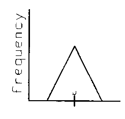
Suppose we had a distribution that was triangle shaped like this:
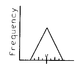
Remember that "µ" is the true average of this population. We would like to have a table showing "how close" the items in the population are to the mean. Two problems arise. First, it would depend on the units used. You would need a different table for acres vs. hectares vs. square miles, etc. Second, the shape may be a triangle, but it could be a short wide triangle or a tall narrow one. Couldn't you replace all these possible tables with just one for any triangular distribution? Of course you could, you just have to measure it cleverly. Let's call ˝ of the base of the triangle "the base unit", and measure areas "around the mean" as percentages of the total population.
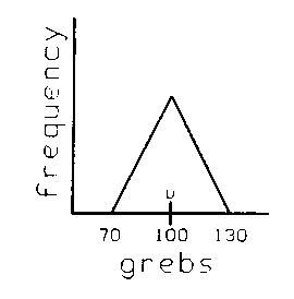
What proportion of the population lies within ± one base unit from the mean? Clearly, 100%. How about ± 0.5 base units on each side of the mean? A bit of math (there are people to do this for us) would tell us 75%. How about ± 0.25 of our base unit? 21.875% is the answer. We now have a short table we can use on any triangular distribution. Suppose we have one like this:
The base unit is clearly equal to "30 grebs" (whatever that is - but it doesn't matter you see). How much of the population is between 85 and 115 (100 ±15) grebs? 75% of course, because ±15 grebs is the same as ±0.5 base units, and we have a table that tells us that. If we were to randomly pick a new item from the population we could say "with 75% confidence" that it would fall within ±0.5 base units, (or in this case ±15 grebs) from the mean. Such an interval could be called "a 75% confidence interval". How much of the population is between 115 and 130? Half of the 25% on the "outside" of the 85-115 range, or 12˝% (the other 12˝% is between 70-85). We have now "standardized" all the possible bases
of triangular distributions into one kind of base unit,
and one table can be made up to tell us all about the
areas under a triangular distribution. We can easily
switch back and forth from base units to real
numbers in grebs, pounds, BF, etc. -- with a little
practice. . | Think about that, and maybe read the previous
section again until it makes sense to you. If you
follow that idea, you can easily understand standard
deviation, confidence intervals, Z tables and a
number of other statistical ideas. It is not a difficult
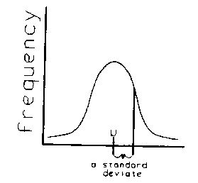
concept. Now to the second distribution -- the "Normal Distribution" or "bell-shaped curve".
This distribution never gets down to the horizontal axis (although it gets very close) so it goes on forever. Because of this, we can't define a base unit in exactly the same way as we did with the triangle, but the idea is the same. Once we had a base unit which would standardize all normal shaped curves (which can also be short and broad or tall and thin like triangles) we would ask somebody to make up a similar table which tells us the percentages under a curve measured by these base units. What should the base unit be? The decision was to use the distance between the mean and the point when the curve stopped curving downward and started curving upward. This point is easy to calculate from the data. We call this base unit a "standard deviate".
When applied to a population it is called "the Standard Deviation of the population" and is given the special symbol (sigma) which you may see on your calculator buttons. It doesn't matter how you calculate it, but how you use it. Want to know how much of a normal curve is between ±1 standard deviation? Look it up in the table, and you get 68%. What table? Well, some nice person has done all the math and called it a Z-table which can be found in most statistics books. You use it just like we did the triangular distribution table to find the probability of any zone under the curve or to create "confidence intervals", usually around the mean. How do you actually calculate this "Standard Deviation" (sigma)? Calculators do that, or computers. You just need to know how to use it. More on that next time. So much for the good news. Now for the bad news. Almost no population is really normally distributed, some not even roughly so. There are thousands of population types, each requiring its own table. In practice we often call anything with one bump in the center and roughly symmetric "Normally Distributed", but this is a lie. So you really can't use the normal distribution on populations, except as a rough approximation. So much for the bad news. Now for the very, very good news. There is a thing called "the Central Limit Theorem", and it says that averages taken from virtually ANY population shape, no matter how weird, very quickly become normally distributed. So averages are always normally distributed, and that is almost always what we are dealing with. Therefore, the thousands of populations can be ignored for most purposes, because the normal distribution always occurs when we sample them. That, gentle readers, is why the "normal distribution" is such a big deal. IT MAKES LIFE SO MUCH SIMPLER. Next time we will talk about how to use this idea to describe the precision of a cruise. |


